BSW Fit
Various options are available for BSW fitting. Basically the teams can add any fitting equation that suits the reservoir engineers. So far, at least three main options are availbale
General Fo Vs Np
The classic function Fo vs Np based on hyperbolic equation.
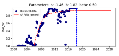
The general equation is:
This will a linear Fo vs Np when beta = 0 (iso exponential):
This will a log linear Fo vs Np when beta = 1 (iso harmonic):
The parameters beta is fixed by best fit using a range (beta min and beta max). The same version but with beta value fixed by the user is under development.
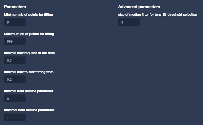
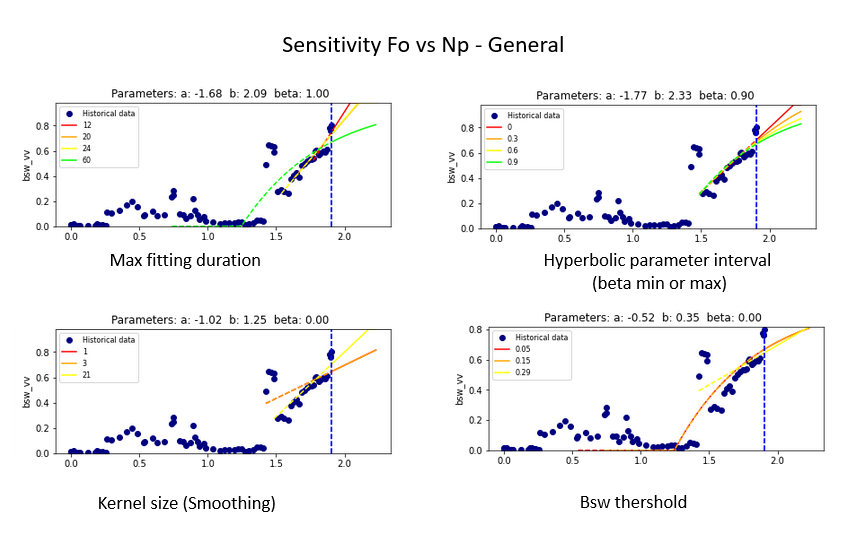
The parameters are as follow: - Minimum / Maximum fitting points: Number of history data (min and max) thay will be used starting from the last point - Minimum BSW: If the bsw historical does not reach this level, the well won’t be forecasted with Fo Vs Np but rather through the next forecaster - Minimum BSW to start fitting the data: It allows to filter the very low values of bsw that are not relevent to the curve (for example bsw < 15%) - Minimum and Maximum beta: Will define the range in which the fit will be performed. if beta = 0 linear if beta =1 log linear. - Kernel size: functionality to smooth bsw curve
Fo Vs Np linear
The same than the previous function but the parameter fixed to 1. Will evolve in the future versions to more genreal values (beta to be fixed by the used)
BSW Fit - Name to be modified
Function developped specilally for Petrocedeno. It allows to fit a simoid function as it is observed in some heavy oil fields a very long bsw plateau after breakthrough
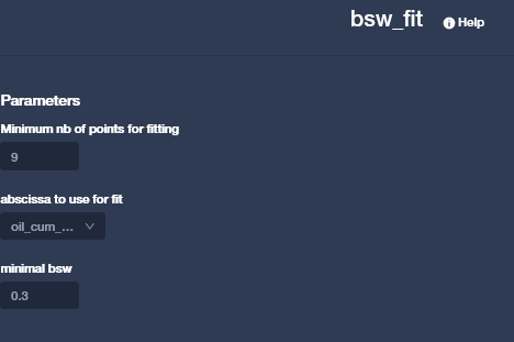
The equation is as follows:
Function will evolve probably in the future