Data Analysis - Curve Types
version - 1.0 (IN PROGRESS)
The purpose of this notebook is to do some basic datanalysis and exploration - it needs the field data - quicklook forecast (or final forecast) in order to analyse the full history of the well
It allows to do: - Computation of curve types - Plots of curve types - Fitting for curve types - Test forecasting based on curve types hypothesis
Library loading:
[1]:
import numpy as np
import pandas as pd
import matplotlib.pyplot as plt
import os
import logging
from frflib.forecast_methods import forecast_wf
from frflib.utils.curve_types import curve_type, plot_curve_type, plot_single_curvetype,merge_category
from frflib.config.config_func import get_var_type
from frflib.config.config_func import get_var_fromvar
from frflib.forecast_tools.datamanip_tools import reindex_df
from frflib.utils.dataframe_func import df_fast_loc
from frflib.plots.utils import get_group_colors
from frflib.utils.curve_types import plot_curve_type
from frflib.forecast_methods.forecast_wf import ForecastWF
from frflib.data_class import input_data
from importlib import reload
import inspect
import frflib
InputData= input_data.InputData
[2]:
PATH_FRFLIB= os.path.dirname(inspect.getsourcefile(frflib))
PATH_TO_DATA= os.path.join(PATH_FRFLIB,"sample_data")
Data Import
[3]:
project_id="01"
wf_name="dataset_01_simple_wf"
WF_PATH=os.path.join(PATH_TO_DATA,f"{wf_name}.hdf")
DATA_PATH=os.path.join(PATH_TO_DATA,f"dataset_{project_id}.hdf")
[4]:
field_data = InputData.load_hdf(DATA_PATH)
wf = ForecastWF.load_from_hdf( WF_PATH, field_data)
field_data._compute_indicators()
wf.enrich_data()
field_data_enriched = wf.enriched_data
[5]:
df_full = wf.get_result_summary(include_stat=True)
If the worklow is going to be applied on a subset of data. It can be extracted using the function subset or a well lsit
## curve type
Parameters
[6]:
groupby_val = ['reservoir']
min_elements = 10
percentile=[0.2,0.5,0.8]
min_active_months=200
[7]:
df_dynamic = wf.enriched_data.df_dynamic
Compute curve type
[8]:
serie_groupby = merge_category(field_data.df_static, groupby_val, min_elements=min_elements)
df_type_curve,df_dyn_resample = curve_type(df_dynamic, serie_groupby, percentile=percentile,min_active_months=min_active_months )
plot result
[9]:
map_colors = get_group_colors(df_type_curve.reset_index(), 'groupby', min_elements=0, select_top=None, color_scale='tab10')
[10]:
plot_curve_type(df_type_curve,var_plots=['oil_rate_stbd', 'oil_cum_mmbbl', 'bsw_vv', 'liq_rate_stbd'],
range_x=[0,20],
color_discrete_map=map_colors)
[11]:
plot_single_curvetype(df_type_curve, df_dyn_resample, group = 'Deltaic',
var_plots = ['oil_rate_stbd', 'bsw_vv', 'gor_vv', 'liq_rate_stbd'],
color_list = ['green', 'blue', 'pink'], percentile = [0.2,0.5,0.8],
range_x = [0,25])
Scatter plot of wells
[12]:
df_plot = df_full.join(serie_groupby).dropna()
[13]:
from frflib.plots.plotly_ import plot_histogram,plot_time_serie, plot_stacked_series, plot_scatter
scatter_param ={
'title': 'Well map - AMAL',
'x_axis': 'x_bh_m' ,
'y_axis': 'y_bh_m',
'x_range': [0.27e+6,0.3e+6],
'y_range': [0.915e+6,0.935e+6], # [2,4.5],
# 'xaxis_type' : None,
# 'yaxis_type' : None, #log
'color' : 'groupby', # 'field'#'sub_group_res' #
'size' : 'max_oil_rate_stbd', #'max_oil_rate_stbd'
'symbol' :'groupby' ,#'reservoir', #"reservoir",# None,
'hover_data':['wellname'],
'same_scale': True,
'height' : 600,
'width' : 900,
'color_discrete_map':map_colors
# 'trendline' : 'ols' #'ols' #None, #'ols'
}
# correct the axis names
plot_scatter(df_plot.reset_index(),**scatter_param)
Export csv
[14]:
filename_export = 'curve_type.csv'
df_type_curve.to_csv(filename_export)
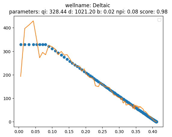
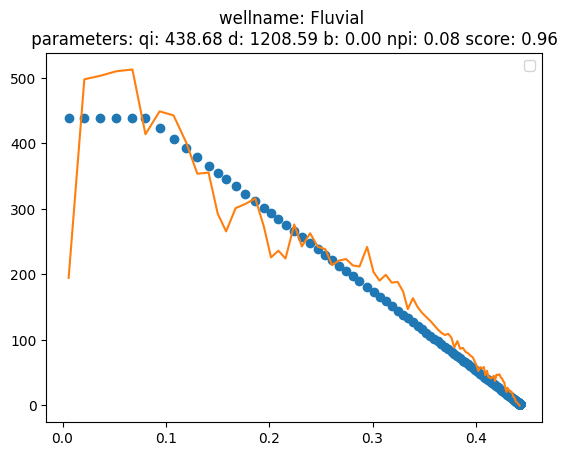
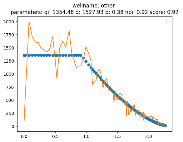
Fit Curve Types
The objective of this section is to fit all the curve types by parameters
[15]:
df_type_curve['P50_oil_cum_mmbbl'] = df_type_curve['P50_oil_rate_stbd'].groupby('groupby').cumsum()*30.5*1e-6
df_type_curve['active_days'] = 25
[16]:
from frflib.forecast_tools.fitters.fitter_catalog import FitDCAHyperPlateau, FitSigmoid
from frflib.forecast_tools.fitters.abs_fitter_class import fit_group, plot_group_fit
FitterClass = FitDCAHyperPlateau
fitter_param = {'min_fit_points':3}
data = df_type_curve #.loc[df_type_curve.count_oil_rate_stbd>2]
x_var = 'P50_oil_cum_mmbbl'
y_var = 'P50_oil_rate_stbd'
df ,fit_dict = fit_group(data, x_var, y_var,FitterClass,**fitter_param)
[17]:
from frflib.plots.matplotlib_ import plot_group_fit
plot_group_fit(df, fit_dict, y_var,x_axis=x_var, well_list='all')
No artists with labels found to put in legend. Note that artists whose label start with an underscore are ignored when legend() is called with no argument.
No artists with labels found to put in legend. Note that artists whose label start with an underscore are ignored when legend() is called with no argument.
No artists with labels found to put in legend. Note that artists whose label start with an underscore are ignored when legend() is called with no argument.
Blind Test Based curve types forecast:
[18]:
wl_list = df_full.loc[df_full.reservoir.isin(['Deltaic'])].index
field_data_nw = field_data.subset(wl = wl_list)
[19]:
# field_data_nw.df_static.loc[field_data_nw.df_static['polygone']=='0']
[20]:
from frflib.forecast_methods import forecast_wf,forecast_new_wf
forecast_new_wf = reload(forecast_new_wf)
ForecastNewWF = forecast_new_wf.ForecastNewWF
[21]:
general_forecast_params = {
'forecast_name': 'wf_ctype',
'forecast_end_date': "01/01/2040",
'forecast_fluids': ['oil','water'],
'forecast_mode': 'blind_test', # 'forecast_mode': 'forecast',blind_test
'abandonned_wells': 5,
'uptime_selection': 'constant_value',
'constant_value': 1.0,
'period_for_avg_months': 12,
'short_term_forecast_adjustment': 0,
'blind_test_duration': 60,
}
para_ctype_nodatefilter = [{
'forecaster_name': 'curve_type_oil',
"learn_x": 'cum_active_days',
'groupby_category': 'reservoir'
},
{
'forecaster_name': 'curve_type_bsw',
"learn_x": 'cum_active_days',
'groupby_category': 'reservoir'
}
]
para_ctype_datefilter = [{
'forecaster_name': 'curve_type_oil',
'early_date_filter': '1/1/2006',
"learn_x": 'cum_active_days',
'groupby_category': 'reservoir'
}
]
Blind test setup:
The idea is to test what would be the forecast for a given number of wells when selecting a curve type based on average behavior. All the wells that started after a certain date will be removed and then forecast based on the group to which they belong It is possible also to filter some wells based on start-up date to take into account only the more recent wells
Blindtest parameters:
[22]:
# wf_ctype_bt_nofilter = ForecastNewWF.execute(field_data_enriched, general_forecast_params, para_ctype_nodatefilter, nproc=1)
# general_forecast_params['forecast_name']= 'wf_ctype_date_filter'
# wf_ctype_bt = ForecastNewWF.execute(field_data_enriched, general_forecast_params, para_ctype_datefilter, nproc=1)
Restults
[23]:
# from frflib.plots.forecast_plots import plot_group_forecast
# y_axis = 'oil_rate_stbd'
# fig_field = plot_group_forecast([wf_ctype_bt, wf_ctype_bt_nofilter], color_list = ['red', 'yellow', 'orange', 'grey'], x_axis='date', y_axis =y_axis)
# fig_field.show()
[24]:
#y_axis = 'water_rate_stbd'
#fig_field = plot_group_forecast([wf_ctype_bt, wf_ctype_bt_nofilter], color_list = ['red', 'yellow', 'orange', 'grey'], x_axis='date', y_axis =y_axis)
#fig_field.show()
Well by well:
[25]:
from frflib.plots.forecast_plots import *
#plot_wells([wf_ctype_bt, wf_ctype_bt_nofilter],x_axis='date', y_axis_list = ['oil_rate_stbd', 'oil_cum_mmbbl'],well_list ='all')
[26]:
#wf_ctype_bt.plot_blind_test()
[27]:
#wf_ctype_bt_nofilter.plot_blind_test()
[ ]: