Assisted Machine learning analysis

The goal of this notebook is to create models to understand the influence of static variables on a dynamic variable. In this example we are going to predict the UER, but any other dynamic variable can be predicted.

If you want more explanations, you can find in the documentation a part dedicated to explain the different concepts.

Import

[1]:

import frflib
import sklearn
from frflib.utils.ml_analysis.optimizer import MLDataset

from frflib.utils.ml_analysis.processing import (
    make_static_list,
    make_pipeline,
    make_dict_preprocessing,
    ONE_HOT_ENCODER,
    TARGET_ENCODER,
    REGROUP_ENCODER,
    XYSCALER,
    MINMAX,
    STANDARD_SCALER,
    UNCHANGED,
)
from frflib.utils.ml_analysis.analysis import (
    find_best_model_param,
    model_analysis,
    fit_model,
    build_model_summary,
)
from frflib.utils.ml_analysis.simulation import (
    get_truncated_normal,
    get_percentile,
    discretize,
    check_enough_data,
    generate_df_simulation,
)
from sklearn.model_selection import train_test_split

from frflib.data_class.input_data import InputData
from frflib.forecast_methods import forecast_wf
from frflib.plots.plotly_ import plot_scatter
import plotly.express as px


ForecastWF = forecast_wf.ForecastWF
import matplotlib.pyplot as plt
import pandas as pd
import numpy as np
import plotly.figure_factory as ff
import plotly.express as px
import os
import inspect
from sklearn.metrics import r2_score, mean_absolute_error, mean_squared_error

/env/lib/python3.8/site-packages/category_encoders/target_encoder.py:92: FutureWarning: Default parameter min_samples_leaf will change in version 2.6.See https://github.com/scikit-learn-contrib/category_encoders/issues/327
  warnings.warn("Default parameter min_samples_leaf will change in version 2.6."
/env/lib/python3.8/site-packages/category_encoders/target_encoder.py:97: FutureWarning: Default parameter smoothing will change in version 2.6.See https://github.com/scikit-learn-contrib/category_encoders/issues/327
  warnings.warn("Default parameter smoothing will change in version 2.6."

Load data

[2]:

PATH_FRFLIB = os.path.dirname(inspect.getsourcefile(frflib))
PATH_TO_DATA = os.path.join(PATH_FRFLIB, "sample_data")

project_id = "01"
wf_name = "dataset_01_simple_wf"

WF_PATH = os.path.join(PATH_TO_DATA, f"{wf_name}.hdf")
DATA_PATH = os.path.join(PATH_TO_DATA, f"dataset_{project_id}.hdf")

[3]:

field_data = InputData.load_hdf(DATA_PATH)
df_st = field_data.df_static
wf = ForecastWF.load_from_hdf(WF_PATH, field_data)
field_data._compute_indicators()
wf.enrich_data()

df_static = field_data.df_static
df_static

[3]:

	production_name	wellbore	reservoir	sub_group	ptr_main_layer_total	ptr_main _layer	ptr_secondary_layer	cluster	avg_poro_vv	avg_vcl_vv	...	z_bh_tvdss_m.1	top_res_sstvd_m	top perfo tvd_ss_ft	z_wh_tvdss_m.1	sensor_depth_tvdss	init_res_pr_bar	init_depletion_pr_bar	start_up_date	year_start	first_prod_days
wellname
well_0	WA12	WA12	Deltaic	B	B22	B2	None	WA	0.54	0.39	...	1077.26	1036.50	1063.72	497.48	962.016	519.86	4.04	2006-12-01	2006	2191
well_1	JD28	JD28	Fluvial	D	D2	D2	None	JD	0.77	0.23	...	1115.73	1003.26	1087.60	332.30	982.500	550.00	1.01	2014-05-01	2014	4899
well_10	SA29	SA29_st1	Fluvial	D	D3	D1	D2	SA	0.64	0.39	...	1295.13	1231.86	1308.72	626.28	1209.727	592.00	4.63	2011-08-01	2011	3895
well_100	RA08	RA08	Fluvial	D	D3	D3	None	RA	0.82	0.26	...	1511.14	1507.18	1444.31	556.99	1329.310	680.00	6.41	2009-03-01	2009	3012
well_101	JB32	JB32_st1	Fluvial	D	D2	D1	None	JB	0.70	0.32	...	1171.23	1105.51	NaN	375.00	NaN	490.00	8.07	2017-01-01	2017	5875
...	...	...	...	...	...	...	...	...	...	...	...	...	...	...	...	...	...	...	...	...	...
well_93	YC13	YC13	Deltaic	B	B22	B2	None	YC	0.68	0.30	...	1166.93	1093.93	1131.87	505.13	1021.972	540.00	4.29	2010-09-01	2010	3561
well_94	VD17	VD17	Deltaic	B	B22	B2	None	VD	0.64	0.40	...	1121.12	1049.24	1101.96	511.04	1039.875	570.00	0.94	2003-03-01	2003	820
well_95	YA18	YA18_st2	Fluvial	E	E1	E1	None	YA	0.51	0.41	...	1452.83	1463.29	1480.16	479.44	1352.500	670.00	5.85	2007-08-01	2007	2434
well_97	P136	P136	Fluvial	D	D3	D3	None	P1	0.74	0.30	...	1301.07	1309.64	1329.15	561.55	1249.500	657.00	2.37	2013-08-01	2013	4626
well_99	P302	P302_st1	Fluvial	D	D3	D3	None	P3	0.73	0.22	...	1320.42	1311.99	1334.13	535.87	1246.300	610.00	5.68	2016-08-01	2016	5722

176 rows × 38 columns

I. Create Model

The first part is to create a model. We are going to choose a model, create a pipeline with some transformations and then train it.

Parameters

The goal is to predict a dynamic variable. You can select here the variable to predict and the models to use. You can add multiple models, but it will take more time. The available models are - gradientBoosting - RandomForest - Lasso - Ridge DATASETS = [“train”, “validation”]

def create_df_result(best_model_dict): model_df = pd.DataFrame() for data_set in DATASETS: data = { key: values for key, values in best_model_dict[data_set].items() if type(values) == list } temp = pd.DataFrame(data=data).set_index(“wellname”) temp[“dataset”] = data_set model_df = pd.concat([model_df, temp], axis=0) return model_df

[4]:

target = "oil_cum_mmbbl"
models = ["GradientBoosting", "Lasso", "RandomForest"]
metric = "neg_mean_squared_error"
availables_metrics = sorted(sklearn.metrics.SCORERS.keys())
assert (
    metric in availables_metrics
), f"metrics not in sklearn metrics please use one of {availables_metrics}"

[5]:

df_predict = field_data.df_dynamic.groupby("wellname").max()
df = pd.concat([df_predict[target], df_static], axis=1)

Cleaning

In this part we drop the wells that didn’t start to produce.

[6]:

df = df.loc[df[target].notnull(), :]

Preprocessing

We have implemented some transformers for basic preprocessing. By default we use the targetEncoder for categorical variable and minmax for numerical data.

All transformers available Categorical - targetEncoder : Replace the categories of categorical columns by the mean of the target - OneHotEncoder

Numerical - XYscaler : scaler to be used with geographical column (x,y) - StandardScaler - minmax : rescale the data between 0 and 1 - unchanged : apply no rescaling on the data

Below you have access to the default a list with each column the default transformer we apply.

If you want to modify the preprocessing, you can follow the below example. You can do 2 things: - don’t keep the column (see example on wellbore below) - Choose another transformer for a column (see example on reservoir)

[7]:

static_col = make_static_list(df.drop([target], axis=1))

col_drop = [
    "gross_lentgh_m",
    "x_wh_m",
    "y_wh_m",
    "z_wh_tvdss_m",
    "z_bh_tvdss_m",
    "z_bh_tvd_m",
    "azim_deg",
    "virgin_res_pr_bar",
    "last_res_pr_bar",
    "z_bh_tvdss_m.1",
    "top perfo tvd_ss_ft",
    "z_wh_tvdss_m.1",
    "sensor_depth_tvdss",
    "init_res_pr_bar",
    "init_depletion_pr_bar",
    "first_prod_days",
    "reservoir.1",
    "ptr_main_layer_total",
    "multi_lateral_flag",
    "ptr_main _layer",
    "ptr_secondary_layer",
    "well_Type",
    "production_name",
    "top_res_sstvd_m",
    "year_start",
    "ptr_main _layer",
    "net_length_m",
    "drill_length_md_m",
    #'reservoir',
    #'wellbore',
    # "avg_vcl_vv",
    # "avg_ntg_vv",
    # "sub_group",
    # "start_up_date",
    # "cluster",
    #'incl_max_deg',
    #'top_res_sstvd_m'
    # "x_bh_m",
    # "y_bh_m"
]
for col in static_col:
    if col["Name"] == "x_bh_m" or col["Name"] == "y_bh_m":
        col["Transform"] = XYSCALER
    if col["Name"] == "reservoir":
        col["Transform"] = ONE_HOT_ENCODER
    if col["Name"] == "top_res_sstvd_m":
        col["Transform"] = MINMAX
    # To choose to delete column from training
    if col["Name"] in col_drop:
        col["Keep"] = False

print("Use in model")
set(df.columns) - set(col_drop)

Use in model

[7]:

{'avg_ntg_vv',
 'avg_poro_vv',
 'avg_vcl_vv',
 'cluster',
 'incl_max_deg',
 'oil_cum_mmbbl',
 'reservoir',
 'start_up_date',
 'sub_group',
 'wellbore',
 'x_bh_m',
 'y_bh_m'}

Pipeline

We then create a sklearndf pipeline with the preprocessing options and the selected models.

[8]:

dict_preprocessing = make_dict_preprocessing(static_col)
preprocessor = make_pipeline(dict_preprocessing)
dict_preprocessing

[8]:

{'numerical': {'minmax': ['avg_poro_vv',
   'avg_vcl_vv',
   'avg_ntg_vv',
   'incl_max_deg'],
  'normalize_standard': [],
  'XYscaler': ['x_bh_m', 'y_bh_m'],
  'unchanged': []},
 'categorical': {'OneHotEncoder': ['reservoir'],
  'targetEncoder': ['wellbore', 'sub_group', 'cluster']},
 'date_time': {'date_time_encoder': ['start_up_date']}}

Fits models

Once the preprocessing is done you can launch the training of the models.

[9]:

# fit on models
# metrics available
# sorted(sklearn.metrics.SCORERS.keys())
# columns = [x["Name"] for x in static_col if x["Keep"] == True]
df_train, df_test = train_test_split(df, test_size=0.3, random_state=35)

data = MLDataset(
    df_train.drop([target], axis=1),
    df_test.drop([target], axis=1),
    df_train[target],
    df_test[target],
)

[10]:

best_model_name, grid, pipe_processor, optimisation_per_model = find_best_model_param(
    data,
    preprocessor,
    metric=metric,
    budget=5,
    models=models,
    feature_selection=False,
    feature_penalisation=False,
)
data_out, model = fit_model(best_model_name, grid, data, pipe_processor)
model_summary = build_model_summary(data_out)
model_summary.update(
    {"optimization_metric": metric, "model": best_model_name, "params": grid}
)
(dict_dependence_plot, dict_summuray_plot, shap_values, df_shap) = model_analysis(
    data_out, model, best_model_name
)

Default parameter min_samples_leaf will change in version 2.6.See https://github.com/scikit-learn-contrib/category_encoders/issues/327
Default parameter smoothing will change in version 2.6.See https://github.com/scikit-learn-contrib/category_encoders/issues/327
Unlike other reduction functions (e.g. `skew`, `kurtosis`), the default behavior of `mode` typically preserves the axis it acts along. In SciPy 1.11.0, this behavior will change: the default value of `keepdims` will become False, the `axis` over which the statistic is taken will be eliminated, and the value None will no longer be accepted. Set `keepdims` to True or False to avoid this warning.
Default parameter min_samples_leaf will change in version 2.6.See https://github.com/scikit-learn-contrib/category_encoders/issues/327
Default parameter smoothing will change in version 2.6.See https://github.com/scikit-learn-contrib/category_encoders/issues/327
Unlike other reduction functions (e.g. `skew`, `kurtosis`), the default behavior of `mode` typically preserves the axis it acts along. In SciPy 1.11.0, this behavior will change: the default value of `keepdims` will become False, the `axis` over which the statistic is taken will be eliminated, and the value None will no longer be accepted. Set `keepdims` to True or False to avoid this warning.

[11]:

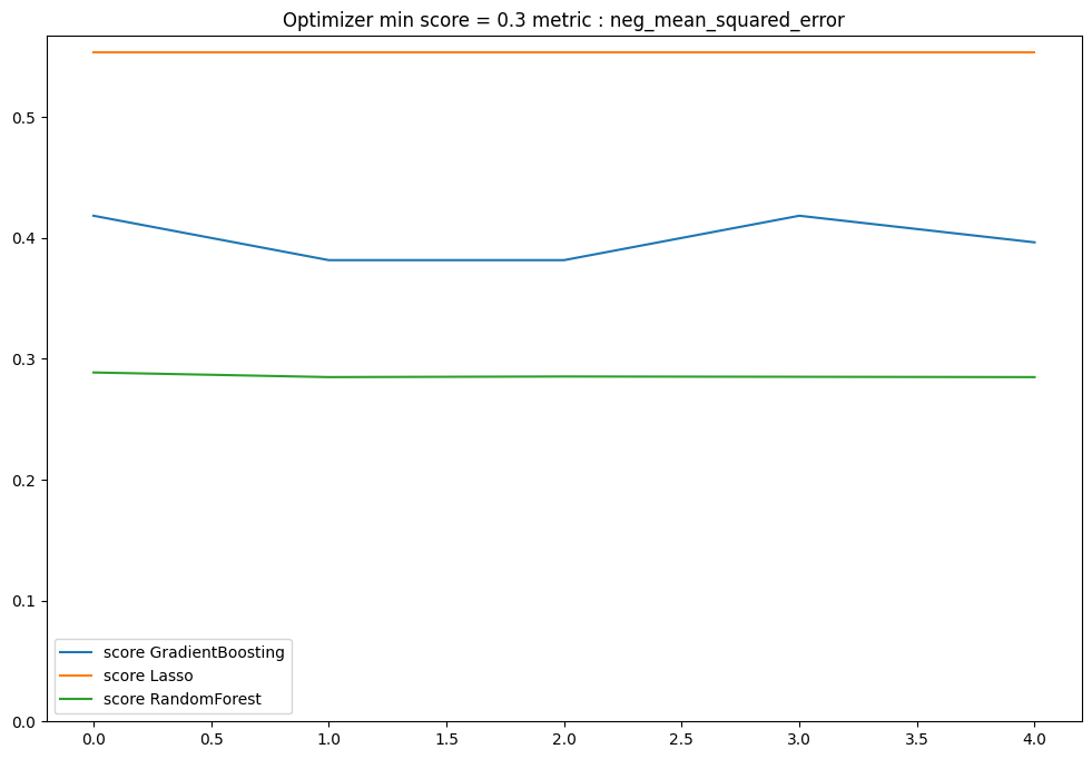
plt.figure(figsize=(12, 8))
for model_name in models:
    score_list = optimisation_per_model[model_name]
    score = [x[0] for x in score_list]
    penalisation = [x[1] for x in score_list]
    plt.plot(score, label=f"score {model_name}")
    if np.sum(penalisation) > 0:
        plt.plot(penalisation, label=f"penalisation {model_name}")
plt.ylim(bottom=0)
plt.legend()
plt.title(f"Optimizer min score = {min(score):.1f} metric : {metric}")
plt.show()

../_images/notebooks_assisted_ml_analysis_21_0.png

II. Model Analysis

Result

Once the preprocessing is done you can launch the training of the models and then visualise the result of the best model. A good indicator is the r2 square. - r2 > 0.6 : really good r2, you have a strong model - 0.6 > r2 > 0.4 : Acceptable r2 - r2 < 0.4 : Low r2, the model is not accurate enough print(f”Best model {model_summary[‘model’]} :nbsphinx-math:`nParams `= {model_summary[‘params’]}”) df_result = create_df_result(model_summary)

metric_func = {“r2”: r2_score, “mae”: mean_absolute_error, “rmse”: mean_squared_error} result_score = {“train”: {}, “validation”: {}}

for dataset in result_score.keys(): original, pred = ( df_result[df_result.dataset == dataset].target, df_result[df_result.dataset == dataset].predict, ) print(f”{dataset}”) for key, func in metric_func.items(): if key == “rmse”: score = func(original, pred, squared=False) else: score = func(original, pred) result_score[dataset].update({key: score}) print(f”\t{key} = {score:.2f}”)

fig_model = plot_scatter( df_result, “target”, “predict”, color=”dataset”, hover_name=”wellname”, same_scale=True, x_range=[0, 70], y_range=[0, 70], title=”Model with all wells”, idendity=True, ) fig_model.show()

[12]:

# inspection
(
    dict_dependence_plots,
    dict_summuray_plot,
    shap_values,
    df_shap,
) = model_analysis(data_out, model, model_name)

Model analysis

Now that we have a model, we are going to make some analysis to understand the influcence of the static variables on the target.

Summuray Plot

This plot gives a summary of the influence and the correlation between the variables and the target. The x-axis is the mean absolute impact on all the wells in term of the target. The variables are sorted according to their impact, and the colour is the correlation (positive or negative with the target).

[13]:

def make_summary_fig(dict_summuray_plot, number_features_plot):
    summuray = pd.DataFrame(data=dict_summuray_plot["data"])
    summuray = summuray[:number_features_plot][::-1]

    fig = px.bar(
        summuray,
        x="mean_abs",
        y="features",
        color="correlation",
        title=f"Impact on {target}",
        orientation="h",
        color_continuous_scale="Bluered",
        range_color=(-1, 1),
    )
    return fig


number_features_plot = 30
fig = make_summary_fig(dict_summuray_plot, number_features_plot=15)
fig.show()

[14]:

# This plot shows the impact of a variable on the target. Compare to the first plot, we can explore each variable at a time. On the x-axis you have the values of the selected variable (which is normalised between [0,1]). On the y-axis you have the impact of the feature. This plot allows us to understand the relationship between the target and variable (linear, monotonic etc…).
df_impact = pd.DataFrame(dict_dependence_plots["data"]).set_index("wellname")
# df_impact = pd.concat([df_impact, df], axis=1)

variable = [x[7:] for x in df_impact.columns if x[:6] == "impact"]
for var in variable[0:2]:
    if f"{var}" in df_impact.columns:
        f = px.scatter(df_impact, var, f"impact_{var}")
        f.show()